Download PDF

Introduction

Choosing the correct curve fit model is crucial when determining important characteristics of data such as the rate of change, upper and lower asymptotes of the curve, or the EC₅₀/IC₅₀ values. The curve fit of choice should represent the most accurate relationship between two known variables: x and y. Therefore, the goal of curve fitting is to find the parameter values that most closely match the data, or in other words, the best mathematical equation that represents the empirical data. SoftMax® Pro 7 Software offers 21 different curve fit options, including the four parameter logistic (4P) and five parameter logistic (5P) nonlinear regression models. These ensure that the plotted curve is as close as possible to the curve that expresses the concentration versus response relationship by adjusting the curve fit parameters of the chosen model to best fit the data.

This technical note discusses the different linear and non-linear regression models available in SoftMax Pro 7. In addition, a protocol has been implemented with the sum of squared errors and the Akaike’s Information Criterion methods in order to evaluate different curve fit models to best represent the data.

Linear regression

The simplest method to analyze data is to use a linear regression curve fit. It is represented by the equation y = A + Bx, where x (generally the concentration) is an independent variable and y (the response) is the dependent variable. The slope of the line is B and A is the y intercept when x=0. SoftMax Pro provides three linear regression curve-fitting methods. These are linear (y = A + Bx), semi-log (y = A + B * log10(x)) and log-log (log₁₀(y) = A + B * log₁₀(x)). SoftMax Pro will find the best straight line through the data (Figure 1). The linear range of an assay can be determined using a minimum of three data points on the x-axis; however, additional standard concentrations within the specified range should be added to improve the accuracy of the fit1. The primary advantage of this method is that it is simple. However, in most cases, the relationship between measured values and measurement variables is nonlinear.

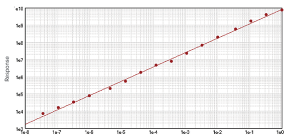
Figure 1. Example of a linear curve fit.

Nonlinear regression

Nonlinear data are commonly modeled using logistic regression. In this case, the relationship between the measured values and the measurement variable is nonlinear. The goal is also to find those parameter values that minimize the deviations between the measured and the expected values. In order to choose the correct fit, it is important to understand the general shape of the model curves and compare them with the shape of the data points².

SoftMax Pro provides 17 non-linear regression curve-fitting methods; these include quadratic, cubic, quartic, log-logit, cubic spline, exponential, rectangular hyperbola (with and without a linear term), two-parameter exponential, bi-exponential, bi-rectangular hyperbola, two site competition, Gaussian, Brain-Cousens, 4P, 5P, and 5P alternate. SoftMax Pro has been implemented with the most widely used iterative procedure for nonlinear curve fitting, the Levenberg-Marquardt algorithm, in order to achieve the best possible curve-fitting.

The two most common nonlinear curve fits are the 4P and 5P, which are sigmoid functions that produce an S shaped curve (Figure 2). They require at least four data points and five data points for the 4P and 5P curve fit model, respectively, but a more accurate fit is obtained by using at least six points for these regression types1. The 4P curve fit is described by the following equation:

y = ((A - D) / (1+ ((x/C)^B))) + D

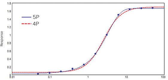
Figure 2. Concentration-response curve fitted with the 4P and the 5P curve fit models for comparison. Although the 4P model gives a smooth symmetrical curve, data are clearly asymmetrical. Therefore, the 5P model gives a better fit.

Where y is the response, D is the response at infinite analyte concentration, A is the response at zero analyte concentration, x is the analyte concentration, C is the inflection point (EC₅₀/IC₅₀), and B is the slope factor. The response increases with concentration if AD. The 4P curve fit is a symmetrical function: one half of the curve is exactly symmetrical to the other half with the EC₅₀/IC₅₀ in the middle.

However, some immuno- and bio-assay data are not symmetrical and need additional flexibility. In those situations, the 5P model may work better as it allows asymmetrical data fitting by adding another parameter, G (Figure 2). The general equation is as follows:

y = ((A - D) / (1 + ((x/C)^B)) ^G) + D

The asymmetry parameter permits each half of the curve to be different. However, when the asymmetry is small, it is advised to use the 4P curve fit model especially if Parallel Line Analysis (PLA) is used in the assay.

Choosing the best curve fit

The overall goodness of the curve fit, particularly the standard curve, should be assessed to obtain accurate and precise data. It is important to run several experiments during the evaluation of a curve fit model as it is difficult to distinguish poor performance from the assay noise in a single run. The R² value is generally a good representation of the goodness of the fit. An R² value is considered a very good fit when it is above 0.99. However, the R² value can be misleading particularly when the standard deviation varies with sample concentration³. Ideally, the standard deviation should be the same at all sample concentrations (homoscedastic data); however, it is not always the case and the standard deviation generally increases with the sample concentration (heteroscedastic data). Methods developed to normalize the data include the Sum of Square Errors (SSE) using the F statistic and the Akaike’s Information Criterion (AIC) methods. Both methods are very similar as they are an assessment of the error between the obtained and the predicted (from the curve fit model of choice) values.

The SSE method is also called the summed square of residuals method as it uses residuals and residual plots (residuals vs. concentration). The residuals are the differences between the response y and the predicted response ŷ obtained from the curve fit model of choice at each concentration⁴: Residual = data – fit = y – ŷ. Residuals represent the random errors. Therefore, when the curve fit model of choice is correct for the data, residuals should appear randomly scattered around the zero line on the residual plot (Figure 3A). If the residuals display a systematic pattern on the residuals plot (Figure 3B), then it is a clear sign that the model fits the data poorly.

Figure 3. Residual plots of data fitted to linear and 4P curve models. (A) The plotted residuals appear randomly scattered around zero indicating that the 4P model describes the data well. (B) The residuals display a systematic pattern showing that the linear model fits the data poorly.

The SSE is obtained using the following formula:

Minimizing the SSE provides a maximum likelihood estimate of the model parameters based on the assumption that data errors are independent and normally distributed. The best curve fit is the one whose parameters generate the smallest SSE. If both models fit the data sensibly, the plot that gives the smallest SSE is the best one to use.

When the two models are nested and one is the special case of the other, e.g. 4P is a special case of a 5P where G=1, the model with the more detailed equation (more parameters) is guaranteed to have a SSE less than or equal to the other model. This is because the model with more parameters will allow more inflection points to fit the data^4. Therefore, some additional statistical calculations, F test and F probability, are needed to determine which model best fits the data. The F probability uses the F test and the degrees of freedom associated with the curve fit model to assess if the decrease in SSE occurred by chance. Typically, a probability below 0.05 (equivalent to 95 % confidence) is used as the threshold and means that the model with the most detailed equation is a better representation of the data.

The AIC method uses a likelihood statistic to compare the goodness of fit of the given data for two curve fit models where one is a special case of the other. The AIC can be calculated using the SSE for data with normally distributed errors as followed:

AIC = n * log (SSE/n) + 2K

where n is the sample size and K is the number of parameters describing the curve. For small sample sizes (i.e., n/K < \~40), the second-order Akaike Information Criterion (AICc) should be used instead:

AIC_c= AIC + 2K ^* (K+1) / (n-K-1)

where n is the sample size and K the number of parameters describing the curve. As sample size increases, the last term of the AIC_c approaches zero and the AIC_c tends to yield the same conclusions as the AIC⁵. The AIC and AICc take into account both the statistical goodness of the fit and the number of parameters that have to be estimated to achieve this particular degree of fit. The AIC penalizes for the addition of parameters and thus selects a model that fits well but has the minimum number of parameters. The curve fit with the lower values of the AIC or AIC_c indicate the preferred model, that is, the one with the fewest parameters that still provides a good fit of the data⁵.

Both methods are useful to determine which curve fit best describes the data, but they do not provide a test of a model in the sense of testing a null hypothesis: i.e they do not give information on the goodness of the fit. If only poor models are considered, it logically selects the best of the poor models. There is an infinite universe of models; curve fitting can find the best parameters for a given model and/or compare two models, but the candidate models should be based on previous investigations and on scientific considerations. After having specified the set of plausible models to explain the data and before conducting the analyses, one should assess the fit of the global model defined as the most complex model of the set. We generally assume that if the global model fits, simpler models will also fit because they originate from the global model^5,6.

Measuring the goodness of the fit

SoftMax Pro 7 has been implemented with a new parameter, Independence, which is one way to examine the suitability of a given curve fit for the data set. The parameter dependency is a measure of the extent to which the best value of one parameter depends on the best values of the other parameters. For a curve fit model of two or more parameters, the parameters describing the curve can be either intertwined (ideal case with an independence of one) or redundant (worst case with independence of zero).

If one parameter is changed after fitting the data with the chosen curve fit, the curve moves away from the data points. If you change the values of the other parameters to compensate for the fixed parameter and the curve moves closer to the points, but with a different curve fit than originally set, then the parameters are intertwined. On the other hand, if the curve goes back to its original position, then the parameters are redundant.

The independence is a number between zero and one with one being the ideal. To display the independence in the graph legend, click on the curve fit settings icon (Figure 4). The curve fit settings window will appear. Simply select the Statistics tab and tick “Calculate Parameter Dependencies”.

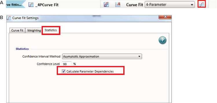
Figure 4. Curve fit display in SoftMax Pro 7. (A) Menu. (B) Curve fit settings.

The graph legend will now display the independence for each parameter describing the curve (Figure 5).

In the graph fit legend in Figure 5, parameter independence has been translated into bars with logarithmic scaling. Ten bars indicate a high degree of independence. Because only very small values indicate a problem, a nonlinear transformation is used for this translation. If one or more parameters have few bars or no bars, the curve fit might not be appropriate for the data set.

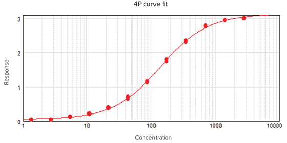
Figure 5. Graph legend showing the parameter independence. The independence is translated into bars where ten bars indicate a high degree of independence.

For example, if the data set was sigmoidal with clear lower and upper asymptotes, a 4P fit would be appropriate with many bars for all parameters. However, if one or both of the asymptotes were missing, the A or the D parameter would have few bars indicating that reliable values couldn’t be deduced from the data set.

Protocol available: Curve Fitting Evaluation

A protocol, Curve Fitting Evaluation, has been developed in SoftMax Pro that automatically calculates the SSE, F probability, and AICc values upon data entry. A result section has been implemented that contains all relevant calculations with the curve fit conclusion using the SSE and AICc methods (Figure 7). The protocol can be downloaded from the SoftMax Pro Protocol Home.

In the following example, data were fitted to a 4P (Figure 6A) and a 5P (Figure 6B) curve fit model which both give an R2 value of 1. All results and calculations were outlined in Figure 7.

Figure 6. Data fitted into curve models. (A) 4P curve fit. (B) 5P curve fit.

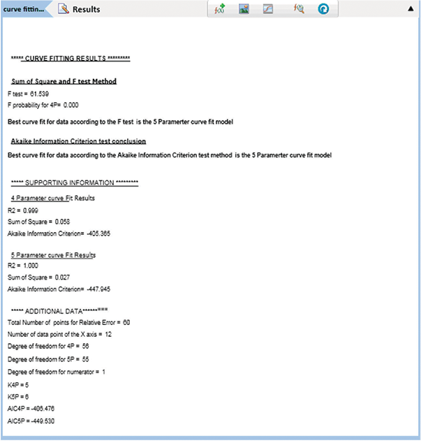
Figure 7. SSE and AICc tests. Results of data fitted into 4P and 5P curve models using the Curve Fitting Evaluation protocol.

The SSE method showed that the 5P curve fit model was a better choice than the 4P for the data with the SSE of 0.058 and 0.027 for the 4P and the 5P curve fit model respectively. The issue was that the 4P curve fit model was a special case of the 5P curve fit model (4P is 5P where G=1). Therefore, the 5P curve fit model was at least as good as a 4P. Additional statistics were needed. The F test (61.539) and F probability (0.000) confirmed that the 5P curve fit model was a better representation of the data than the 4P curve fit model in this example. The AIC_c method also showed that the 5P offered a better fit to the data than the 4P curve fit model: AICc of -405.365 for the 4P and -447.945 for the 5P curve fit model. Finally, the residual plot had residuals randomly scattered around the zero line and confirmed that either curve fit model was correct for the data (Figure 8). Taken together, the test methods indicated that the 5P curve fit model was a better fit to the data.

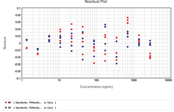
Figure 8. Residual plot for data fitted into 4P and 5P curve models.

Summary

A wide range of mathematical models are available in SoftMax Pro 7 including the widely used 4P and 5P curve fit models. The R² value can be a poor measure of the curve fit quality for the data, particularly for heteroscedastic data. The SSE with the F probability and the AIC_c methods are useful to compare the goodness of the fit and to choose the best possible curve fit model with confidence. However, the first step is to make sure that both models fit the data with sensible values and make scientific sense. SoftMax Pro 7 includes a method of calculating the parameter dependency to estimate the goodness of a curve fit. The resulting parameter independence is visually displayed in the graph legend to help interpret your data easily.

References

1. Davis D, Zhang A, Etienne C, Huang I, and Malit M. Principles of curve fitting for multiplex sandwich immunoassays. Rev B Tech Note 2861. In. Bio-Rad Laboratories, Inc, Hercules, CA. 2002.
2. Ledvij M. Curve fitting made easy. The Industrial Physicist. 2003; 9:24-27
3. Kiser MM and Dolan JW. Selecting the best curve fit. LC-GC Europe. March 2004; 138-143
4. Gottschalk PG and Dunn JR. The 5-Parameter Logistic: A characterisation and comparison with the 4-Parameter logistic. Analytical Biochemistry. 2005: 343:54-65.
5. Burnham KP and Anderson DR. Model Selection and Multimodel Inference: a practical information-theoretic approach. 2nd edition. New York: Springer-Verlag, 2002.
6. Cooch EG and White GC. Program MARK: Analysis of data from marked individuals, a ‘gentle introduction’. www.phidot.org/software/mark/docs/book. 2001.

Learn more about SoftMax Pro 7 Software >>

Download PDF